Building a Retrieval-Augmented Generation (RAG) system is exciting until you look at the bill. You’ve got Large Language Models that are expensive to run, vector databases storing millions of chunks, and embedding services processing terabytes of data. It’s easy to assume every part of this pipeline is costing you a fortune. But here’s the reality check: most of your money isn’t going where you think it is.
If you’re trying to slash costs by switching to cheaper embedding models or tweaking your vector store settings, you might be missing the forest for the trees. The real savings lie in understanding the hierarchy of expenses in a production RAG pipeline. Let’s break down exactly where your budget goes and how to optimize each layer without sacrificing quality.
The Real Cost Hierarchy of RAG Systems
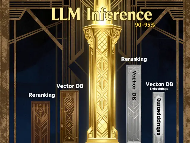
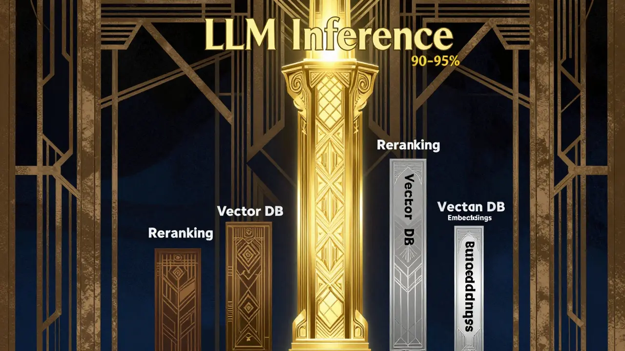
Before optimizing anything, you need to know what actually drives your spend. According to analysis from CostLens.dev, the cost structure of a typical RAG deployment is heavily skewed. LLM inference accounts for 90-95% of total operational costs. That’s right-nearly all your money is spent on the final step where the model generates the answer.
Reranking services consume 3-7%, vector database operations take 1-2%, and embedding generation is less than 1%. This hierarchy changes everything. Optimizing an already-cheap component like embeddings yields negligible savings compared to reducing the tokens sent to the LLM. Your primary job-to-be-done should be maximizing value from those expensive inference tokens, not obsessing over pennies saved in storage.
- LLM Inference: 90-95% of costs. High impact.
- Reranking: 3-7% of costs. Medium impact.
- Vector DB Ops: 1-2% of costs. Low impact.
- Embedding Generation: <1% of costs. Minimal impact.
Optimizing Context Budgets: The Highest Impact Lever
Since LLM inference dominates your bill, reducing the context window size passed to the model is your single most effective cost-saving strategy. Every token you cut from the prompt saves money directly. Here’s how to shrink that context without losing relevance.
First, minimize the quantity of retrieved documents. Instead of fetching ten relevant chunks, fetch three highly relevant ones. Second, implement intelligent document reranking. A reranker scores initial results and prioritizes the best passages, allowing you to pass fewer, higher-quality chunks to the LLM. This often justifies the 3-7% cost of reranking because the subsequent LLM token savings exceed the reranking expense.
Third, truncate retrieved content. Strip out headers, footers, and boilerplate text before sending chunks to the model. Finally, use hierarchical retrieval strategies that progressively refine context based on relevance scores. Even modest reductions in token count yield significant savings. If you can reduce your average context length by 20%, you’re cutting nearly 20% off your largest expense line item.
Smart Embedding Model Selection
While embedding costs are low, choosing the wrong model can still bloat your storage and slow down ingestion. OpenAI’s text-embedding-3-small costs $0.02 per million tokens with 1536 dimensions, while text-embedding-3-large costs $0.13 per million tokens with 3072 dimensions. For 10,000 documents averaging 500 tokens, the small model costs $0.10, and the large model costs $0.65. Both are cheap, but the large model doubles your storage footprint.
| Model | Price per 1M Tokens | Dimensions | Batch Latency |
|---|---|---|---|
| text-embedding-3-small | $0.02 | 1536 | ~500ms |
| text-embedding-3-large | $0.13 | 3072 | ~800ms |
For many domain-specific applications, smaller specialized models outperform larger general-purpose ones. A 384-dimensional model reduces storage by 62.5% compared to a 1024-dimensional one while maintaining comparable retrieval quality. Evaluate models across semantic quality, dimensionality, inference speed, and total cost. Don’t default to the biggest model; choose the smallest one that meets your accuracy threshold.

Advanced Storage Optimization: Quantization and PCA
When storage costs start adding up, especially with millions of vectors, you can compress embeddings without losing much performance. Research published on arXiv (2505.00105v1) evaluated various strategies on the MTEB benchmark. The standout winner? Float8 quantization.
Float8 achieves a 4x storage reduction compared to float32 baseline while keeping performance degradation below 0.3%. It outperforms int8 quantization at equivalent compression ratios and is simpler to implement. Combine this with Principal Component Analysis (PCA) for even greater savings. Moderate PCA-based dimensionality reduction retaining 50% of original dimensions, combined with float8 quantization, achieves 8x total compression.
This combined approach performs better than int8 quantization alone despite achieving double the compression ratio. Use the formula: Storage (bytes) = N × (Original Dimensions × PCA Ratio%) × Bytes per Dimension. For example, reducing 1536 dimensions to 768 via PCA and then applying float8 quantization drastically shrinks your vector database footprint. This is particularly useful if you’re using serverless vector stores like Pinecone, which charge $0.25 per gigabyte per month for storage.
Pipeline Efficiency: Deduplication and Incremental Processing
Your data ingestion pipeline can silently waste resources. Duplicate and near-duplicate content inflates processing requirements and skews retrieval results. Implement source-level deduplication to remove duplicates before processing. Post-chunking, use algorithms like MinHash or SimHash to detect near-duplicate chunks before embedding. This saves both embedding generation costs and storage capacity.
Adopt incremental processing strategies. Use content hashing to identify only new or modified documents, avoiding reprocessing static knowledge base portions. Avoid re-embedding unchanged content by tracking checksums or modification dates. Batch process document embeddings rather than handling them one-at-a-time. Frameworks like sentence-transformers support batch operations with CUDA acceleration, significantly improving GPU utilization and reducing per-document overhead.
Index Tuning and Response Caching
Vector database index optimization offers secondary performance gains. Common index types include HNSW (Hierarchical Navigable Small World) and IVF_FLAT (Inverted File with Flat Clustering). HNSW parameters like ef_construction and M affect build time, storage overhead, query speed, and accuracy. Tune these to align with your specific deployment needs. Some configurations incur additional storage overhead through auxiliary data structures, so balance speed against space.
Don’t overlook response caching. Store previously computed responses for identical or semantically similar queries. High-traffic RAG systems often experience sufficient query repetition patterns that caching eliminates redundant LLM inference costs entirely. This is a high-return optimization that requires minimal architectural changes but can dramatically lower your monthly bill.
Monitoring and Pareto-Optimal Configuration
To manage costs systematically, track key metrics: volume of raw data processed, number of chunks generated, total storage size, ingestion pipeline runtimes, and API costs. Use cloud provider budget tools to set alerts when expenditures approach thresholds. This proactive monitoring prevents surprise bills.
Select configurations using a Pareto-optimal framework. Plot achieved retrieval performance (e.g., nDCG@10) against required storage size. Each point represents a unique combination of embedding model, quantization type, and PCA level. Identify your target memory constraint line, then select the configuration achieving the highest performance score within that budget. This ensures you’re getting the best possible quality for your specific storage limits.
Is it worth switching to a cheaper embedding model?
Probably not. Embedding costs account for less than 1% of total RAG expenses. Switching models yields negligible savings. Focus instead on reducing LLM context size, which drives 90-95% of costs.
What is the most effective way to reduce RAG costs?
Reduce the context window size passed to the LLM. Use reranking to select fewer, higher-quality chunks, truncate unnecessary text, and employ hierarchical retrieval strategies. This directly cuts the most expensive part of your pipeline.
How does float8 quantization help?
Float8 quantization reduces storage by 4x compared to float32 with less than 0.3% performance loss. Combined with PCA, it can achieve 8x compression, significantly lowering vector database storage costs without hurting retrieval quality.
Should I use HNSW or IVF_FLAT indexes?
It depends on your trade-offs between query speed, build time, and storage overhead. HNSW generally offers faster queries but may have higher storage overhead due to auxiliary structures. Tune parameters like ef_construction and M to match your specific latency and accuracy requirements.
Does reranking increase costs?
Yes, reranking adds 3-7% to costs, but it usually pays for itself. By improving retrieval quality, it allows you to pass fewer, more relevant chunks to the LLM, saving significant inference costs that outweigh the reranking expense.